Waves and swells

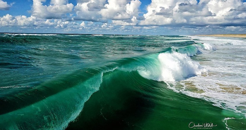
The waves that we see propagating on the surface of oceans, seas or lakes are usually caused by wind. Waves can also be generated by a moving body in the water, such as bow waves. The displacement of the ocean floor due to an earthquake or an underwater landslide can also create a long wave of the tsunami type. Let’s focus on wind-driven waves and try to understand their various shapes. This will lead us to use certain words from the marine vocabulary such as fetch and to understand both the varied, more or less irregular shapes of their surface and the mechanisms of their propagation. Why do some waves break, possibly forming the superb rollers sought by surfers? What happens below the surface and how deep is the water agitated? How can the energy of these waves be evaluated and captured?

1. From waves to regular swells

Wave propagation generally represents the response of a physical medium to a disturbance. A restoring force then tends to bring the medium back to equilibrium. In the case of acoustic waves, this is the compressive strength of the medium (See: The emission, propagation and perception of sound). In the case of a liquid surface, two forces are involved: gravity and surface tension. The latter leads to the propagation of small ripples on a centimetre scale, but the waves and swells that interest us here are entirely governed by gravity. Gravity tends locally to bring the free surface back to its horizontal equilibrium shape, but this movement induces pressure forces which transmit the movement to the surrounding water, and thus propagate the disturbance.

Waves are generated by the wind through complex mechanisms that are still under investigation. However, when they move away from their generation zone, waves become more regular and are then referred to as swell. This swell can be described as a sum of elementary sinusoidal waves which lend themselves well to mathematical analysis.

Figure 1: Wave channel and its wavemaker [Source: © LEGI]

 

Such regular swells are reproduced in basins by oscillating mechanical wavemakers (Figure 1). The parameters that control their behaviour can then be set: their period and amplitude, as well as the water height of the basin.

2. Low amplitude swell

The amplitude of the swell is defined as the maximum deviation of the surface from its horizontal equilibrium shape. It is equal to half the total height H between the crest and trough (Figure 2). The notion of “low” amplitude refers to the wavelength λ, i.e. the slope of the surface remains low. The amplitude should also be small in relation to the water height d.

In this small amplitude limit, the fluid mechanics equations admit simple solutions, of sinusoidal form. This is called an Airy swell, named after the British mathematician and astronomer George Biddell Airy (1801-1892).

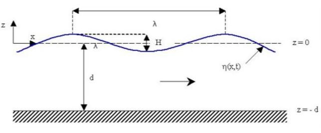
In addition to its amplitude, this swell is characterized by its period T (the duration of an oscillation at a given point) and its wavelength λ (the distance between two successive peaks). The wavelength is related to the period by the propagation speed c=λT, which depends on the water height according to a formula given by the mathematical solution.

In the case of deep water (relative to the wavelength), the propagation velocity is expressed as where g is the acceleration of gravity. A swell of wavelength λ=10 m thus propagates at speed c=4 m/s, and a swell of wavelength λ=100 m propagates faster, at speed c=12.5 m/s. The corresponding periods, T=λ/c, are T=2.5 s and T=8 s respectively. Combining these formulas we can also express the wavelength as λ=gT²/ (2π).

The other limiting case corresponds to shallow water, for which the wavelength is large compared to the depth d. In this case the wave propagates at the velocity independent of the wavelength. For example, a tsunami propagates with a characteristic length of the order of a hundred km, large compared to the ocean depth of a few km. It is then in the shallow water regime, and for d=4 000 m, the propagation speed c=200 m/s. The tide also propagates on the surface of the Earth as a shallow water wave, with a main period of 12 h, and a corresponding wavelength of several thousands of km (Read: Tides).

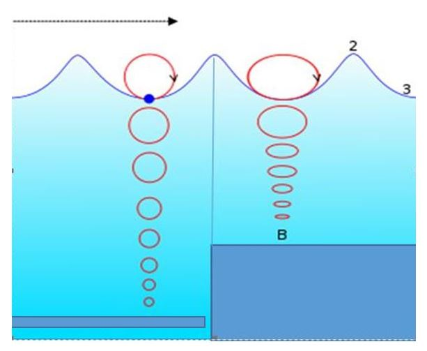
The speed of propagation of the wave should not be confused with the speed of displacement of the water particles, which is much lower and gives a circular trajectory for the particles in deep water (see Figure 3). For particles located at the free surface, the diameter of the trajectory is equal to the total height H of the swell. The fluid velocity is thus equal to πH/T, significantly smaller than the propagation velocity λ/T for a sinusoidal swell. The diameter of these trajectories tends exponentially to 0 with depth, becoming practically zero at a depth equal to half a wavelength.

In shallow water these trajectories become elliptical and flatten towards the bottom, the horizontal component being of great importance for sediment transport.

These trajectories are closed, and the average displacement of a fluid particle is therefore zero. However, this is only a first approximation, valid only in the limit of a very low amplitude wave. The particles in fact move a distance of the order of 40H²/λ per period. This is called the Stokes drift, named after the British mathematician George Gabriel Stokes (1819 -1903) who described and calculated it. For a swell of height H=2m and wavelength λ=100 m the displacement is thus 1.6 m per period.

3. Non-linear swells

The sinusoidal swell is only a first approximation valid for low amplitudes. We then speak of “linear swells” corresponding to the simplified form of the equations of motion, known as “linear”. In this approximation, any wave field can be described as an addition of elementary sinusoidal waves, each keeping its identity.

Apart from linear Airy swells, two types of non-linear swells can be distinguished:

• swells of greater amplitude in deep water
• swells in shallow water

The domain of validity of the different wave regimes are shown in Figure 4 as a function of the amplitude H and water depth d, related to the wave period T to form the parameters H/gT² and d/gT². Knowing that the wavelength in deep water is expressed as λ=gT²/(2π) for a sinusoidal wave, these two parameters actually compare respectively the wave height and the depth to this wavelength. The bottom of the graph corresponds to the linear limit of low amplitudes, where the waves are sinusoidal.

3.1. Deep water swell

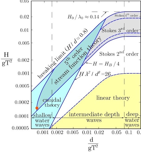
The right-hand side of the graph in Figure 4 corresponds to deep water, for which more complex periodic mathematical solutions were obtained by the mathematician George Gabriel Stokes mentioned earlier. The 2^nd, 3^rd, or 4^th order Stokes waves correspond to increasing amplitudes, which move us further and further away from the sinusoidal case: the troughs become more and more spread out, and the peaks more and more acute, until they form an angular vertex (of angle 120°). At this point the wave becomes unstable and breaks up by breaking. Its curvature represented by the ratio H/l reaches a limit value of about 0.14, and beyond this limit amplitude, there is no more periodic swell: it breaks.

3.2. Shallow water swell

The domain of shallow water swells, corresponds to the left part of Figure 4.

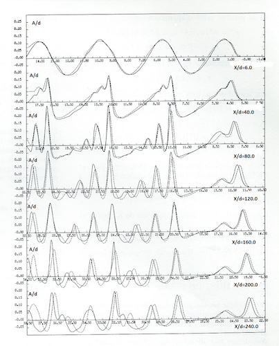
Figure 5 (solid line) shows the evolution of an initially sinusoidal swell propagating in a horizontal bottom swell channel. The water height is d=10 cm, while the initial wave height is H=2.5 cm and its period T=4 seconds, giving a wavelength of 4 meters. The relative depth d/gT² is therefore equal to 0.0006 and the relative height H/gT² to 0.00015, which is represented by the red dot in Figure 4. This puts us well into the shallow water domain.

Each solid line curve gives the time evolution of the height at different relative distances x/d from the origin where the wave is produced by an oscillating wavemaker (like the one shown in Figure 1). Rapidly each initial period breaks down into a sequence of peaks of decreasing amplitude and decreasing velocity. Thus the main peak of each period can catch up with the secondary peaks of the previous period.

Stockes’ theories, even at higher orders, give a poor representation of these phenomena. A better mathematical representation of wave propagation in shallow water uses non-linear equations (K D V equations) named after the scientists who studied them: Korteweg (1848-1941) and De-Vries. In Figure 5 a numerical simulation (dashed line) of the wave propagation using these equations is in very good agreement with the recordings.

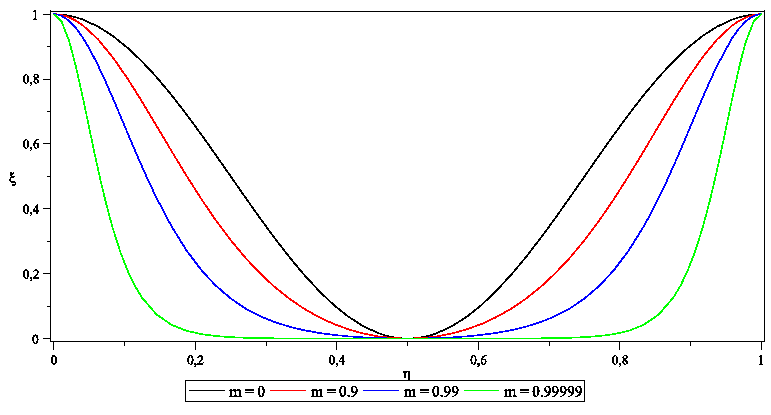
4. Cnoidal swell and solitary waves

The K-D-V equations admit periodic solutions called “cnoidal waves” [1] for which their asymmetry becomes considerable, until they can form isolated peaks called “solitary waves”. Such profiles can be seen in Figure 6. At very low amplitude the cnoidal wave tends to be sinusoidal.

Solitary waves have the remarkable property of forming spontaneously from milder initial conditions as seen in Figure 5. In nature, this is the case of an earthquake in a maritime area which generates a tsunami wave of the order of a metre offshore. This wave is amplified when the water depth near the coast decreases and decomposes into a train of solitary waves whose amplitude can reach about twenty meters. Such waves then become devastating and deadly as was the case in Japan with 23,500 deaths (2015) and in Indonesia with over 200,000 deaths (2004). (Read: Tsunamis, knowing them to better predict them)

5. Modification of the swell as it approaches a beach

During their propagation, swells can undergo modifications due to the morphology of the coastline or the topography of the sea bed. When it meets a wall or a steep coastline, the swell undergoes a reflection. In the case of a cape, the swell can then change its direction of propagation by the phenomenon of diffraction, which can be seen in Figure 7.

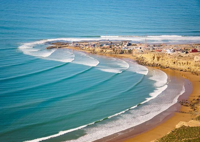
The swell is also deflected by a change in depth, due to the refraction phenomenon. Thus, when approaching a beach, the crest lines tend to follow the bathymetric lines [2], as can be seen in Figure 7. This effect is due to the decrease in swell velocity at shallower depths. Similarly, light is deflected when entering a medium with a high refractive index, where it propagates more slowly.

The swell crest rises more and more as it approaches the beach, until it breaks. This effect is due to the decrease in propagation speed for a constant energy flow, which implies an increase in energy density, and therefore in wave height, as well as a decrease in wavelength. At shallow depths, the wave crest propagates faster than the troughs, which leads to the final break.

The impact of the swell on a beach leads to a slight rise in elevation, called a run-up, which can induce currents back out to sea, a source of danger for bathers.

It can happen that swell trains arrive from different directions and by interaction give cross swells or a embossed sea. Figure 8 shows a embossed sea in shallow water where the relatively regular swells have a cnoidal profile with a trough more elongated than the crest; a slight reflection near the coast appears.

Finally, the swell is influenced by the coastal morphology, but also sculpts the shoreline in the long term, by the erosion of rocky coasts and beaches, as well as by the deposition of sediments according to the currents it induces.

6. Sea swells and wind generation

The wind blowing on the sea surface transfers part of the energy from the atmosphere to the water surface. This is a phenomenon of friction between the layers of air and water, which creates depressions on the crests and overpressures in the troughs, amplifying the initial wavelets to form a complex regime of waves that become longer and more powerful as they propagate.

In deep water the parameters involved are the wind speed, the length of the area where the wind blows, called the fetch, and the duration of the wind. The depth of the water will also have an influence if it is shallow. For example, a wind blowing at 15 m/s for 10 hours on a fetch of about 100 km generates waves of significant height Hs (see definition below) of about 3 m. Note that the wind speed increases with height: the reference speed, noted U10, is the one measured at 10 meters above the sea (in average position).

7. Irregular swells

Outside of the fetch area, the waves will smooth out and become less rough, while still retaining their irregular swell character (see Figure 9).

There are two ways to analyze them: local statistical analysis and spectral analysis.

7.1. Local statistical analysis

The profile of a real swell is usually very complex. The total height and period are calculated by decomposing the profile into a succession of elementary waves. There are two possibilities to evaluate the height (Figure 10):

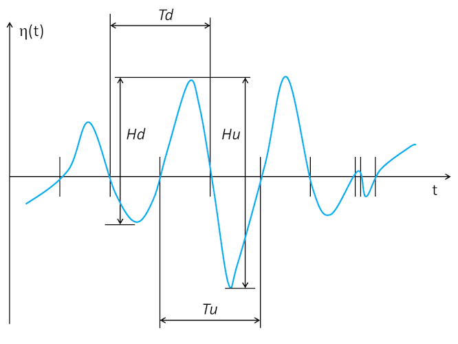
• the height from a trough to the next crest is called downcrossing and noted H_d ;
• from a peak to the next trough is the upcrossing height noted H_u.

The average values of H_d and H_u are the same and give an estimate of the total height H. We do the same for the period with T_d and T_u to have an estimate of the period T.

In practice, we are more interested in what is called the significant height H_s which corresponds to the average value of the heights of the third highest waves [3]. The marine meteorology gives H_s which is calculated by numerical modelling from the spectrum of the swell, knowing the wind speed and the fetch (see 7.2). In shallow coastal areas the model also incorporates the bottom topography.

7.2. Spectral analysis

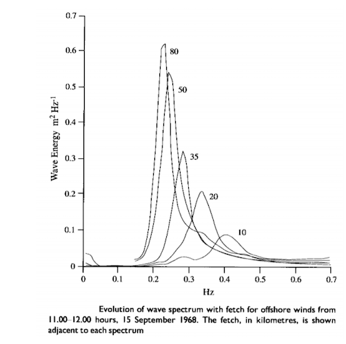
Spectral analysis is another way to statistically describe a wave train. It involves representing the distribution of wave energy as a function of frequency. One of the most common spectral representations is the so-called JONSWAP spectral function, whose name originates from the analysis of data from measurements made at sea during the Joint North Sea Wave Project [4]. The curves depend on parameters representing the wind speed and the fetch which are at the origin of the waves (Figure 11). The graphs show that in the wind action zone, the waves become progressively stronger in energy (amplitude), while evolving towards lower frequencies, which corresponds to longer waves.

7.3. Rogue wave

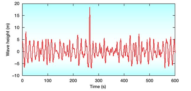
Sometimes a very large wave (two to three times Hs), called a rogue wave, appears in the middle of a wave train. The accounts of this phenomenon observed by various sailors have long been questioned. However, modern recording methods have confirmed this reality. Figure 9 shows the signal of a rogue wave with a height of about 26 metres in a wave train of significant amplitude Hs of 11.8 metres. This recording was made on 01/01/1995 on the Draupner oil platform off Norway. A wave is qualified as a rogue wave when it appears in an isolated way in the middle of a wave train with an amplitude of more than 2 times higher than the significant amplitude of this train. It is estimated that 22 cargo ships sank between 1973 and 1994 due to rogue waves, causing hundreds of casualties [5].

The origin of a rogue wave is not yet well understood and could be explained by non-linear interactions or by the meeting of wave trains of different origins. However, scientists have been able to carry out a laboratory experiment that shows a rogue wave resulting from the crossing of two wave trains at an angle of 120 degrees [6].

8. Wave energy

Is the energy given up by the wind to the wave recoverable? This is a question that has become very important in recent years in the context of renewable energy research. An approximation formula allows us to calculate the power E (energy supplied per second) per linear metre of peak, E=0.5H_s²T  (kW/m). Approximately 2% of the 800,000 km of world coastline have an average energy power greater than 30 kW/m, which corresponds to a total power of about 0.5 TW [7], or an annual production of electrical energy of about 2,000 TWh (8% of world consumption) [8].

Knowing that it is not feasible to develop all these coasts, the possible contribution to global power generation remains limited, but can be of great interest locally, especially for the many existing islands around the world. This has led in recent decades to the development of various techniques to recover this energy. Projects have been completed or are underway to test the cost-effectiveness of these techniques and several hundred patents have been filed. Insertion in coastal protection schemes presents particularly attractive opportunities.

Some projects are based on the oscillating water column principle. This type of installation (Figure 12) consists of a concrete box immersed in water, open to the sea at the bottom (1) and whose free surface inside is in contact with a volume of air (2). The reciprocating movement of the sea level causes the air inside the caisson to compress and decompress, thereby activating a turbine (3) which produces electricity.

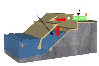
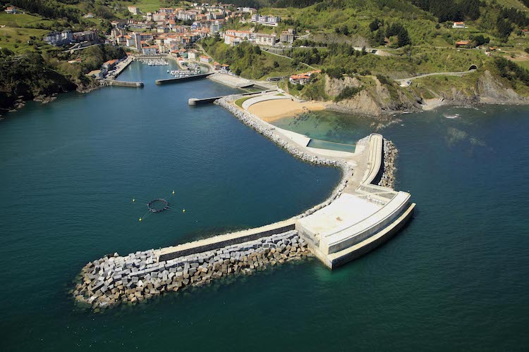
A pre-commercial prototype was built in Mutriku in the Bay of Biscay by the Basque Energy Agency and commissioned in 2011. This 300 kW wave power plant is incorporated in a breakwater (Figure 13).

9. Message to remember

• Waves are generated by the wind in the fetch area;
• Outside the fetch zone, the waves smooth out to give more or less regular swells;
• In the vicinity of the coastline, the swells are deformed under the influence of variations in bathymetry and coastal morphology.
• In coastal areas, in combination with currents, swells have a fundamental importance on sediment transport.
• Wave energy can be partly recovered.

---

Notes and references

Cover image. [Source: VIGNA christian, CC BY-SA 4.0, via Wikimedia Commons]

[1] These solutions involve Jacobi elliptic functions noted cn, hence the adjective “cn-oidal”.

[2] Lines of equal depth, equivalent to the level lines for the reliefs (from the ancient Greek bathys meaning “deep”)

[3] This height Hs given by weather reports is about 4 times the standard deviation of the vertical surface deviation η (the standard deviation is the square root of the mean of η2). The precise relationship between these two quantities is, however, complex and depends on wind conditions.

[4] Hasselmann et al (1973) Measurements of wind-wave growth and swell decay during the Joint North Sea Wave Project (JONSWAP), Ergnzungsheft zur Deutschen Hydrographischen Zeitschrift Reihe, A(8) (Nr. 12), p.95.

[5] https://fr.wikipedia.org/wiki/Vague_sc%C3%A9l%C3%A9rate

[6] Allister et al. (2019) Laboratory recreation of the Draupner wave and the role of breaking in crossing seas, J. Fluid Mechanics 860, 767-786.

[7] The terawatt (TW) is a unit of power that corresponds to 10¹² watts or one billion kilowatts. One TWh is the total energy supplied by 1 TW for one hour (or 3600 terajoules).

[8] www.irena.org/Publications/2014/wave-énergie